Regression Model Development (part 2)

Regression Model Development (part 2)#

Processing Categorical Data (the right way)#

In the previous section, we avoided the additional complexity of processing categorical data by simply removing it. While this sped things along, it also dropped potentially valuable insight from our analysis. Now that the code is working, we’ll rebuild our models using that categorical data -the type feature.

df_sample = df.sample(n=10, random_state = 152)
# df_sample_highlight = pd.concat([df_sample.iloc[:5,:], df_sample.iloc[-5:,:]]).style.format().set_properties(subset=['type'], **{'background-color': 'yellow'})

# function definition
def highlight_cols(s):
    color = 'null'
    if s == 'Iris-virginica': color = 'limegreen'
    elif s == 'Iris-setosa': color = 'lightblue'
    elif s == 'Iris-versicolor': color = 'orange'
    # color = 'red' if s == 'Iris-virginica' or 'blue' if s == 'Iris-setosa'
    return 'background-color: % s' % color
  
# highlighting the cells
df_sample.style.applymap(highlight_cols)

	sepal-length	sepal-width	petal-length	petal-width	type
38	4.400000	3.000000	1.300000	0.200000	Iris-setosa
115	6.400000	3.200000	5.300000	2.300000	Iris-virginica
36	5.500000	3.500000	1.300000	0.200000	Iris-setosa
122	7.700000	2.800000	6.700000	2.000000	Iris-virginica
21	5.100000	3.700000	1.500000	0.400000	Iris-setosa
7	5.000000	3.400000	1.500000	0.200000	Iris-setosa
89	5.500000	2.500000	4.000000	1.300000	Iris-versicolor
48	5.300000	3.700000	1.500000	0.200000	Iris-setosa
51	6.400000	3.200000	4.500000	1.500000	Iris-versicolor
127	6.100000	3.000000	4.900000	1.800000	Iris-virginica

We have three mutually exclusive flower types, equally distributed, in this feature:

df.groupby('type').size().plot(kind='pie',colors = ['lightblue', 'orange', 'limegreen']);

A piechart is shown. The graph is split into three equal groups + Orange = Iris-versicolot, green = Iris-virginica, and blue = Iris-setosa.

Recall, a coding [error was returned](sup_reg_ex: develop: train) after inputting this data directly into linear_reg_model.fit. This occurred because the algorithm did not how to process categorical independent variables. This isn’t a problem when using dependent categorical variables for classification models as in our classification example. Those algorithms are written to expect dependent categorical variables -as they always classify categories.

But algorithms like numbers and there are many instances when ML models can only interpret numerical data. Furthermore, how categories should be represented requires an understanding of the data. Something the algorithm doesn’t have. Thus feature encoding, processing data into numerical form, is an essential data analytical skill. To do this properly you should understand your data before preceding.

For example, we could simply re-label the types as follows:

\[\begin{split} \text{Iris-setosa} \rightarrow 1 \\ \text{Iris-versicolor} \rightarrow 2 \\ \text{Iris-virginica} \rightarrow 3 \\ \end{split}\]

and hand this off to the algorithm. While this would fix the coding error, any mathematical interpretation of this re-labeling would be meaningless, e.g., Iris-setosa is not twice as much as Iris-versicolor, nor does setosa + versicolor = virginica -the type is just a name. We call this type of categorical data nominal. Categories with an inherent order, e.g., grades, pay grades, bronze-silver-gold, etc., are called ordinal. But that doesn’t apply here either. A flower either is an Iris-setosa OR it isn’t. Each type is similarly binary so we can interpret each unique type as a unique feature, with a 1 or 0, indicating whether the category applies or not.

Most machine learning libraries are equipped with built-in preprocessing functions; see the available options in the docs: sklearn.preprocessing. For simplicity, we’ll start with Pandas’ built-in get_dummies. However, it will often be best to use functions specifically written for your model’s library, such as sklearn’s OneHotEncoder.

after_pd_dummy = pd.get_dummies(df_sample)

Before
	type
38	Iris-setosa
115	Iris-virginica
36	Iris-setosa
122	Iris-virginica
21	Iris-setosa
7	Iris-setosa
89	Iris-versicolor
48	Iris-setosa
51	Iris-versicolor
127	Iris-virginica

After *get_dummy*
	type_Iris-setosa	type_Iris-versicolor	type_Iris-virginica
38	1	0	0
115	0	0	1
36	1	0	0
122	0	0	1
21	1	0	0
7	1	0	0
89	0	1	0
48	1	0	0
51	0	1	0
127	0	0	1

This process is called vectorization. Now we can include type in the training and testing of a model:

from sklearn.model_selection import train_test_split
from sklearn.linear_model import LinearRegression 
from sklearn.metrics import mean_squared_error

X = pd.get_dummies(X)
X_train, X_test, y_train, y_test = train_test_split(X, y, test_size=0.333, random_state=41)
linear_reg_model_types = LinearRegression()
linear_reg_model_types.fit(X_train,y_train)
y_pred = linear_reg_model_types.predict(X_test)

sme = mean_squared_error(y_test, y_pred)
print('MSE using types is :' + str(sme))

MSE using types is :0.12921261168601364

When including the flower types, our linear model has a mean squared error of \(\approx 0.129\). Recall from the previous section without the flower types, we had a MSE of abot \(0.123\).

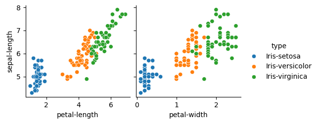
So did it get worse? No. Our data changed and you can’t simply compare MSE’s from different cases. Converting types to numerical features, added three dimensions to the previous example. Moving from three to a *six-*dimensional space. Consider the change from just two to three dimensions, e.g., \(2^{2}=4\) to \(2^{3}=8\). Adding dimensions can radically increase the volume of space making the available data relatively sparse -what’s known as the Curse of Dimensionality. -However, that’s not the full story here. While, both petal-length and petal-width appear positively correlated with sepal-lengthfor versicolor and virginica it does not for setosa (blue below),

import seaborn as sns

#correlogram
sns.pairplot(df,x_vars = ['petal-length','petal-width'], y_vars=['sepal-length'], hue='type');

Two scatterplots are shown side by side. The y-axis for both is sepal-length. The x-axis is petal-length and petal-length for the left and right plot, respectively. Both plots similarly show positive linear correlations for the color-coded Iris-versicolor and Iris virginica data points. The Iris-setosa data points are grouped in the lower-left quadrant of both plots with little linear correlation.

The drop in accuracy is in part a limitation of our simple linear model trying to make use of a feature pulling the model in the wrong direction. Making the most out of your data involves a mix of understanding the data and the applied algorithm(s) (which don’t understand anything). Using three different linear models yields better results:

from sklearn.model_selection import train_test_split
from sklearn.linear_model import LinearRegression 
from sklearn.metrics import mean_squared_error


df_dummy = pd.get_dummies(df)
df_dummy
df_s = df_dummy.loc[df_dummy['type_Iris-setosa'] == 1].drop(columns=['type_Iris-versicolor', 'type_Iris-virginica'])
df_v = df_dummy.loc[df_dummy['type_Iris-versicolor'] == 1].drop(columns=['type_Iris-setosa', 'type_Iris-virginica'])
df_g = df_dummy.loc[df_dummy['type_Iris-virginica'] == 1].drop(columns=['type_Iris-setosa', 'type_Iris-versicolor'])

def line_regression_pipe(df_list):
    for df in df_list:
        X = df.drop(columns=['sepal-length']) #indpendent variables
        y = df[['sepal-length']].copy() #dependent variables
        #split the variable sets into training and testing subsets
        X_train, X_test, y_train, y_test = train_test_split(X, y, test_size=0.333, random_state=41)
        linear_reg_model_a = LinearRegression()
        linear_reg_model_a.fit(X_train,y_train)
        y_pred = linear_reg_model_a.predict(X_test)
        sme = mean_squared_error(y_test, y_pred)
        print('MSE of ' + df.columns[4] + ' is :' + str(sme) )

df_list = [df_s, df_v, df_g]
line_regression_pipe(df_list)

MSE of type_Iris-setosa is :0.06604867484155268
MSE of type_Iris-versicolor is :0.09862408497975977
MSE of type_Iris-virginica is :0.0802189108860733

The goal of this section was to illustrate how to incorporate independent categorical variables. Though it starts with converting strings to numbers, how those conversations are done is important to consider. Moreover, the introduction of more features can impact both the computational efficiency and accuracy of the model.

Regression Model Development (part 2)

Contents

Regression Model Development (part 2)#

Processing Categorical Data (the right way)#