Data Exploring and Processing

Here we’ll do two essential things.

1. Process the data.

2. Analyze the data.

Processing will involve importing, cleaning, and sorting raw data; preparing it to be analyzed. Exploring the data builds an understanding of it and the problem you’re trying to solve, equipping you to develop a machine-learning application.

Before doing anything with raw data, you must import it.

# We'll import libraries as needed, but when submitting, 
# it's best to have them all at the top.
import pandas as pd

# Load this well-worn dataset:
url = "https://raw.githubusercontent.com/jbrownlee/Datasets/master/iris.csv"
df = pd.read_csv(url) #read CSV into Python as a DataFrame
df # displays the DataFrame

	5.1	3.5	1.4	0.2	Iris-setosa
0	4.9	3.0	1.4	0.2	Iris-setosa
1	4.7	3.2	1.3	0.2	Iris-setosa
2	4.6	3.1	1.5	0.2	Iris-setosa
3	5.0	3.6	1.4	0.2	Iris-setosa
4	5.4	3.9	1.7	0.4	Iris-setosa
...	...	...	...	...	...
144	6.7	3.0	5.2	2.3	Iris-virginica
145	6.3	2.5	5.0	1.9	Iris-virginica
146	6.5	3.0	5.2	2.0	Iris-virginica
147	6.2	3.4	5.4	2.3	Iris-virginica
148	5.9	3.0	5.1	1.8	Iris-virginica

149 rows × 5 columns

Oops.* The first row of data has been set as headers. Some data sets have headers already -this one doesn’t. How do we fix that? Google “how to python add headers to dataframe”. You’ll need to learn a lot of micro-skills -pick them up when needed. Reading up on the data set, Iris flower data set, we name the columns:

column_names = ['sepal-length', 'sepal-width', 'petal-length', 'petal-width', 'type']
df = pd.read_csv(url, names = column_names) #read CSV into Python as a DataFrame
df # displays the DataFrame

	sepal-length	sepal-width	petal-length	petal-width	type
0	5.1	3.5	1.4	0.2	Iris-setosa
1	4.9	3.0	1.4	0.2	Iris-setosa
2	4.7	3.2	1.3	0.2	Iris-setosa
3	4.6	3.1	1.5	0.2	Iris-setosa
4	5.0	3.6	1.4	0.2	Iris-setosa
...	...	...	...	...	...
145	6.7	3.0	5.2	2.3	Iris-virginica
146	6.3	2.5	5.0	1.9	Iris-virginica
147	6.5	3.0	5.2	2.0	Iris-virginica
148	6.2	3.4	5.4	2.3	Iris-virginica
149	5.9	3.0	5.1	1.8	Iris-virginica

150 rows × 5 columns

Supervised methods use “answers” in the data to supervise the model. Does our data contain the “answers”? If we want to predict the Iris ‘type,’ then yes. It’s the only categorical feature, so we’ll go with it. However, a supervised method could predict any of the features, e.g., ‘sepal-length.’ A supervised method can’t predict what it doesn’t have, say, plant height or petal color.

What? That’s it for data processing? We didn’t do much becasue the data didn’t need much. Like a lot of data out there, it was (mostly) ready to go. No minimal processing is required. The project’s needs determine the required data processing, i.e., if it works, you’ve done enough. See Data Requirements.

That’s all the processing needed for now.

Descriptive Methods and Visualizations

Let’s explore the data. A good starting question: how many different Iris categories do we have?

num_types = df.groupby(by='type').size();
display(num_types); 

type
Iris-setosa        50
Iris-versicolor    50
Iris-virginica     50
dtype: int64

Let’s visualize that with a bar plot.

#Using Pandas plot.bar 
plot = num_types.plot.bar(color=['red','blue','green'],rot=0)

Want to do something similar but different? Go to the libary’s docs. You’ll see many libraries and functions each with lots of options. Don’t just copy, paste, and pray. Read the docs and understand the parameters.

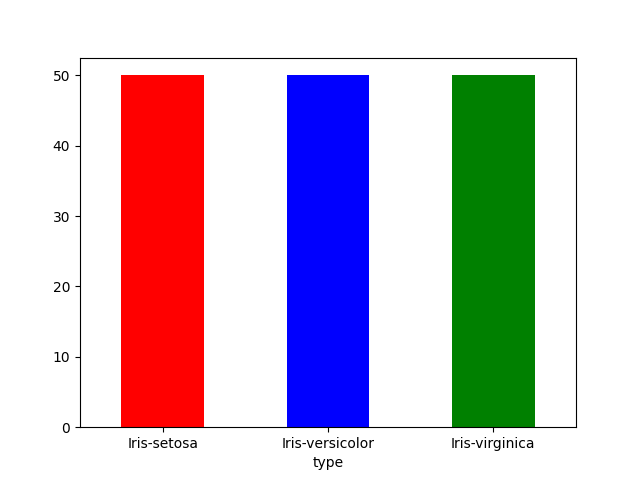
Three evenly distributed categories. What about the distribution of the petal widths? As with most things in nature, we might expect it to be somewhat normal.

hist_petal_lengths = df['petal-length'].hist(grid = False,bins=10, legend = True)

Not so normal. However, we are looking at the petal lengths of all three types. So let’s look at a single type.

df_typeA = df[df['type'] == 'Iris-setosa']
df_typeA['petal-length'].hist(grid = False, color = 'red');

df_typeA['petal-length'].hist(grid = False, color = 'red');
plot_with_alt_text('A histogram showing the distribution of petal-length for the Iris-setosa typer. There are 10 bins ranging 1-2 (x-axis).' \
                   + 'The y-axis is the number in each bin ranging 0-14.' \
                   + 'There is one grouping appearing normally distributed an x-range of approximately = [1.0, 1.95] and a y-range of approximately = [0, 14].')

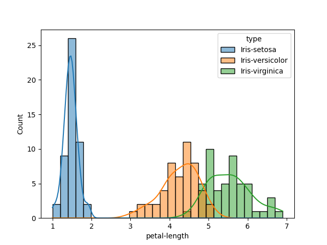
Evaluators don’t assess aesthetics, but Pandas’ visualizations are limited compared to others. Below we get a much better picture of what’s going on, and we clearly see the three different types.

A histogram to visualize distributions:

import matplotlib.pyplot as plt
import seaborn as sns

sns.histplot(df,x='petal-length', hue='type', kde=True, bins =30);

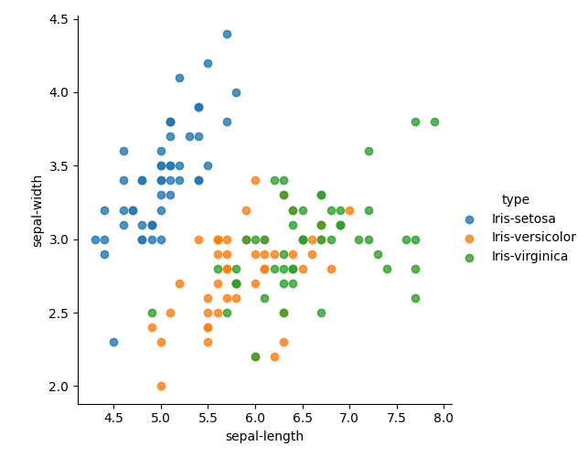
A scatterplot to visualize popssible correlations:

#https://seaborn.pydata.org/generated/seaborn.lmplot.html
sns.lmplot(x='sepal-length', y='sepal-width', data=df, fit_reg=False, hue='type')
plt.show()

A correlogram to visualize distributions and correlations of and between multiple variables.

#correlogram. https://seaborn.pydata.org/generated/seaborn.pairplot.html#seaborn.pairplot
sns.pairplot(df, hue='type')
plt.show()

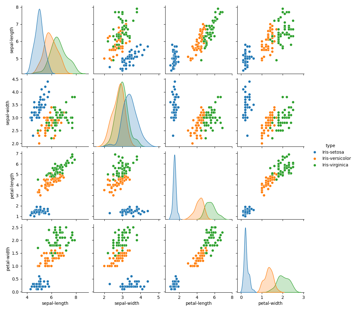
Each image is a descriptive method and a visualization (\(\geq3\) meets the requirements). And here are some non-visual descriptions of the data:

df.describe(include='all')

	sepal-length	sepal-width	petal-length	petal-width	type
count	150.000000	150.000000	150.000000	150.000000	150
unique	NaN	NaN	NaN	NaN	3
top	NaN	NaN	NaN	NaN	Iris-setosa
freq	NaN	NaN	NaN	NaN	50
mean	5.843333	3.054000	3.758667	1.198667	NaN
std	0.828066	0.433594	1.764420	0.763161	NaN
min	4.300000	2.000000	1.000000	0.100000	NaN
25%	5.100000	2.800000	1.600000	0.300000	NaN
50%	5.800000	3.000000	4.350000	1.300000	NaN
75%	6.400000	3.300000	5.100000	1.800000	NaN
max	7.900000	4.400000	6.900000	2.500000	NaN

Play around -explore.