Example: Supervised Regression App

To predict a number for a feature contained in the data, use a supervised regression method (but not logistic regression).

For this example, we’ll slightly modify the previous example. Instead of predicting the category type, we’ll predict the number sepal-length.

Show code cell source Hide code cell source

#We'll import libraries as needed, but when submitting, 
# it's best having them all at the top.
import pandas as pd

# Load this familiar dataset:
url = "https://raw.githubusercontent.com/jbrownlee/Datasets/master/iris.csv"
df = pd.read_csv(url) #read CSV into Python as a DataFrame

#Attach column names to the dataframe
column_names = ['sepal-length', 'sepal-width', 'petal-length', 'petal-width', 'type']
df = pd.read_csv(url, names = column_names) #read CSV into Python as a DataFrame
pd.options.display.show_dimensions = False #suppresses dimension output

##preserves Jupyter preview style (the '...') after applying .style
def display_df(dataframe, column_names, highlighted_col, precision=2):
    pd.set_option("display.precision", 2)
    columns_dict = {}
    for i in column_names:
        columns_dict[i] ='...'
    df2 = pd.concat([dataframe.iloc[:5,:],
                       pd.DataFrame(index=['...'], data=columns_dict),
                       dataframe.iloc[-5:,:]]).style.format(precision = precision).set_properties(subset=[highlighted_col], **{'background-color': 'yellow'})
    pd.options.display.show_dimensions = True
    display(df2)
    
#display df with highlighted column 
display_df(df, column_names, 'sepal-length', 1)

	sepal-length	sepal-width	petal-length	petal-width	type
0	5.1	3.5	1.4	0.2	Iris-setosa
1	4.9	3.0	1.4	0.2	Iris-setosa
2	4.7	3.2	1.3	0.2	Iris-setosa
3	4.6	3.1	1.5	0.2	Iris-setosa
4	5.0	3.6	1.4	0.2	Iris-setosa
...	...	...	...	...	...
145	6.7	3.0	5.2	2.3	Iris-virginica
146	6.3	2.5	5.0	1.9	Iris-virginica
147	6.5	3.0	5.2	2.0	Iris-virginica
148	6.2	3.4	5.4	2.3	Iris-virginica
149	5.9	3.0	5.1	1.8	Iris-virginica

The highlighted numbers, ‘sepal-length,’ provides something to predict (dependent variables), and the non-highlighted columns are something by which to make that prediction (independent variables). The big differences from the previous example are as follows:

• Data processing (maybe) if we choose to include type as an independent variable, it’ll need to be converted from categorical data into numbers the model can use.

• Model Development As we’ll be predicting a number, a regression method will be used instead of a classification method.

• Accuracy Metric instead of a simple percentage, we’ll need a measurement of how close the data fits the model. e.g., mean squared error.

Data Exploring and Processing

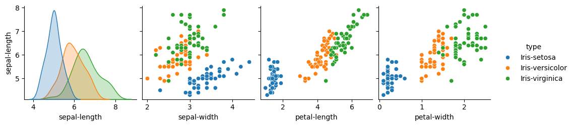
As the data is identical, this step will be similar to what was done in the previous example; please refer to it. Focusing on the sepal length, we can certainly see patterns:

Show code cell source Hide code cell source

import matplotlib.pyplot as plt
import seaborn as sns

#correlogram
sns.pairplot(df, y_vars=['sepal-length'], hue='type')
plt.show()